Yarrr

Author

geonaumov@ioworx.net

YaRrr! The Pirate’s Guide to R

by Nathaniel D. Phillips

URL: https://bookdown.org/ndphillips/YaRrr

The dataset

suppressPackageStartupMessages(library(circlize))
library(yarrr)

Loading required package: jpeg

Loading required package: BayesFactor

Loading required package: coda

Loading required package: Matrix

************
Welcome to BayesFactor 0.9.12-4.7. If you have questions, please contact Richard Morey (richarddmorey@gmail.com).

Type BFManual() to open the manual.
************

# message("SUMMARY:")
# summary(pirates)
message("COLUMNS:")

COLUMNS:

names(pirates)

 [1] "id"              "sex"             "age"             "height"         
 [5] "weight"          "headband"        "college"         "tattoos"        
 [9] "tchests"         "parrots"         "favorite.pirate" "sword.type"     
[13] "eyepatch"        "sword.time"      "beard.length"    "fav.pixar"      
[17] "grogg"

# knitr::kable(head(pirates), format="markdown")

A dataset containing the results of a survey of 1,000 pirates.

Some calculations

Calculate the mean age, separately for each sex

sex_agg <- aggregate(x = age ~ sex, data = pirates, FUN = mean)
knitr::kable(sex_agg, format="markdown")

sex	age
female	29.92241
male	24.96735
other	27.00000

Create a scatter plot

plot(x = pirates$height,
     y = pirates$weight,
     main = 'A scatter plot',
     xlab = 'Height',
     ylab = 'Weight',
     pch = 16,
     col = gray(.0, .1))

Linear regression model

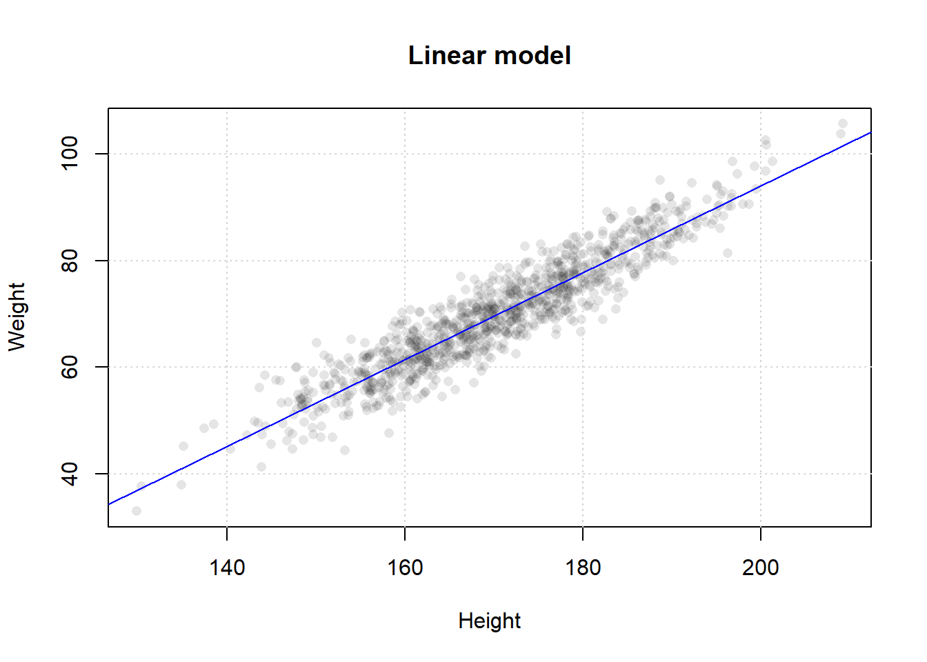
plot(x = pirates$height,
     y = pirates$weight,
     main = 'Linear model',
     xlab = 'Height',
     ylab = 'Weight',
     pch = 16,
     col = gray(.0, .1))

grid()
model <- lm(formula = weight ~ height, data = pirates) # Linear model
abline(model, col = 'blue')

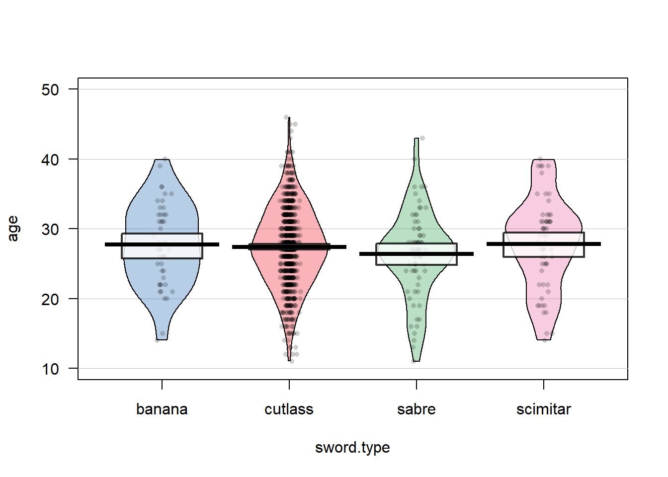
Pirate plots

Ages by favorite sword

pirateplot(formula = age ~ sword.type, 
           data = pirates)

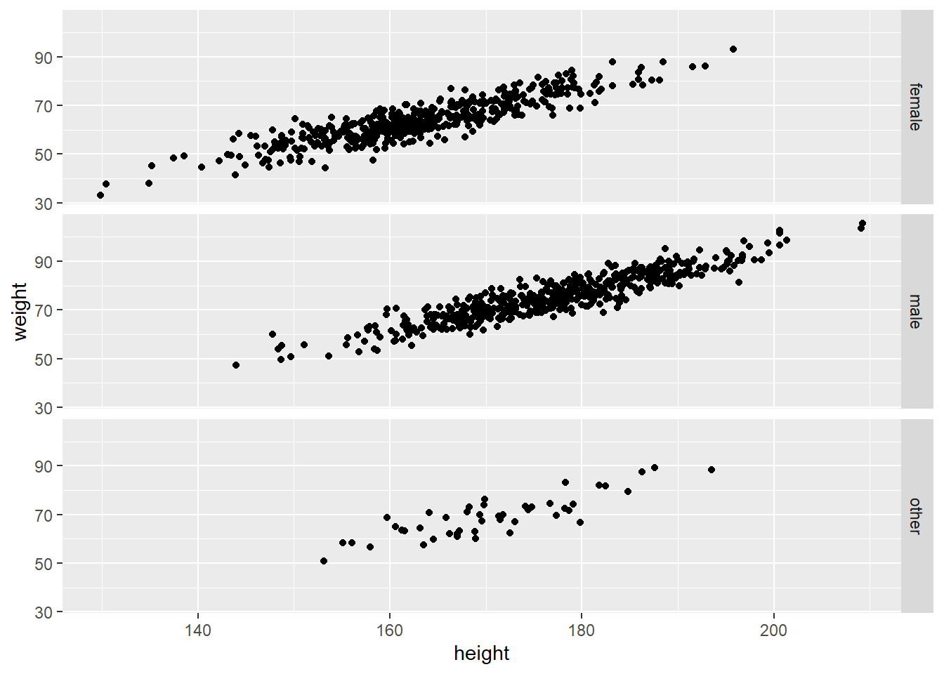
Weight and height vs sex

library(ggplot2)


Attaching package: 'ggplot2'

The following object is masked from 'package:yarrr':

    diamonds

p <- ggplot(pirates, aes(height, weight)) + geom_point()
p + facet_grid(rows = vars(sex))

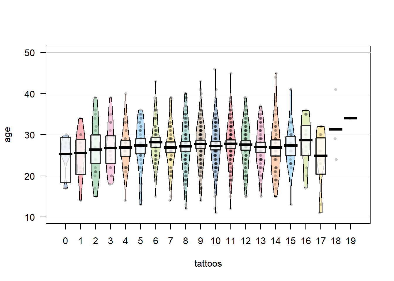
Ages by tattoots

pirateplot(formula = age ~ tattoos, 
           data = pirates)

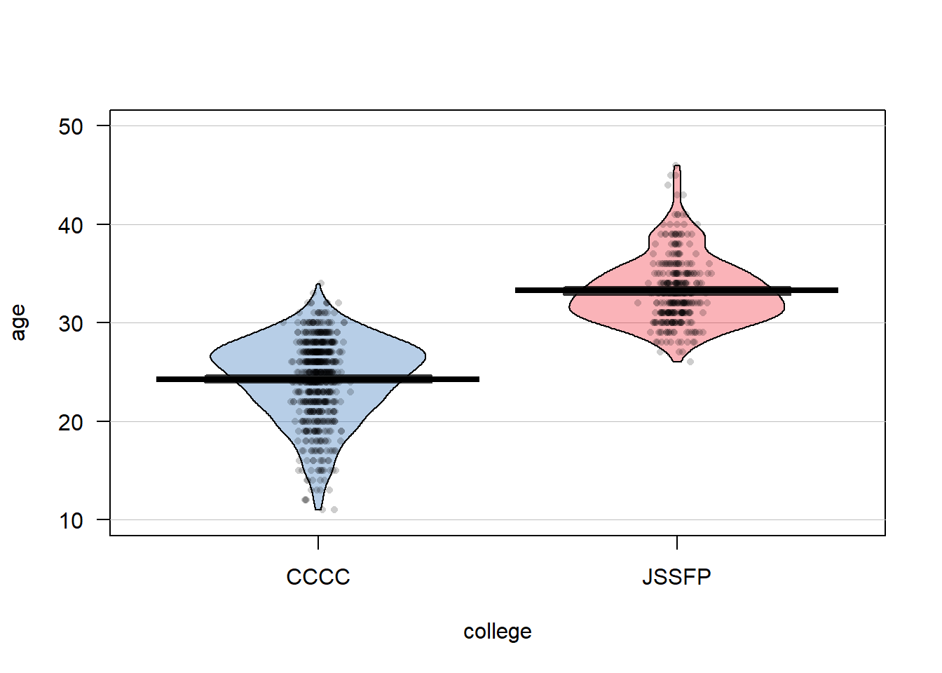
Ages by college

pirateplot(formula = age ~ college, 
           data = pirates)

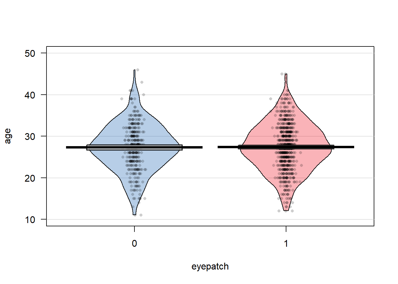
Ages by eyepatch

pirateplot(formula = age ~ eyepatch, 
           data = pirates)

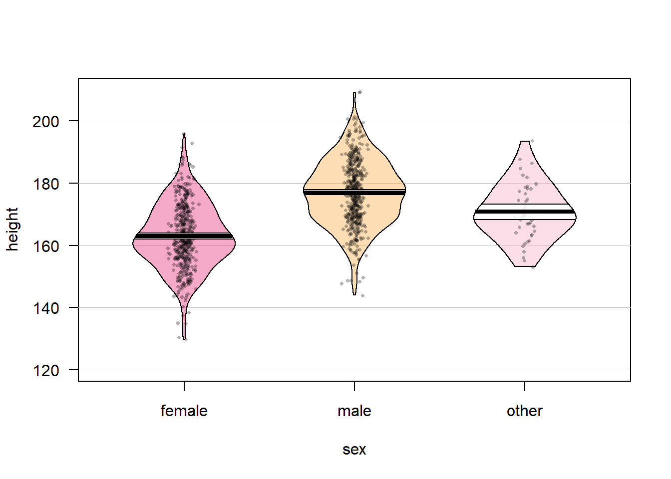
Height by sex

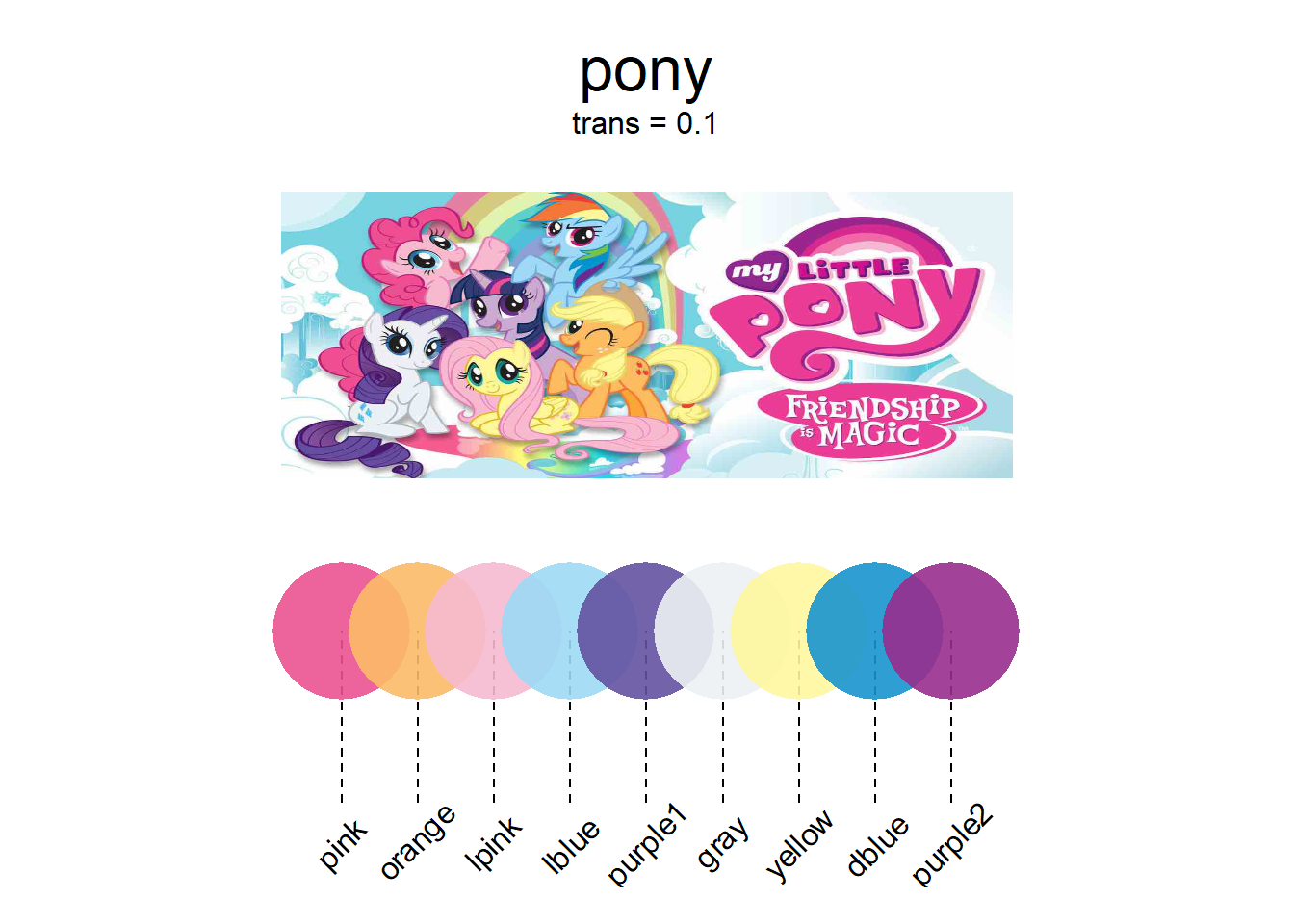
pirateplot(formula = height ~ sex,               # Plot weight as a function of sex
           data = pirates,                       
           pal = "pony",                         # Use the info color palette
           theme = 3)                            # Use theme 3

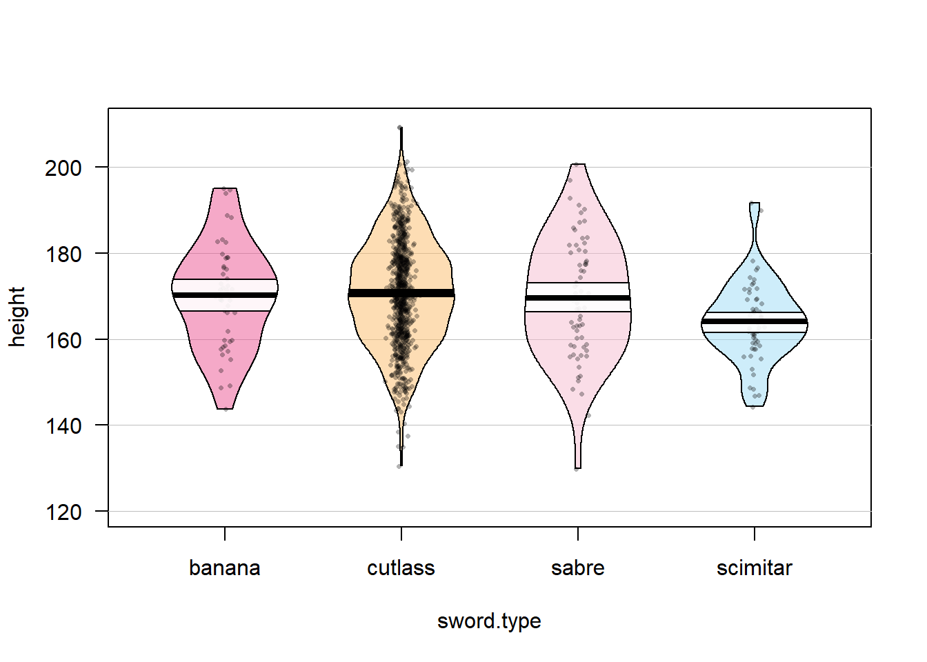
Height by fav. weapon

pirateplot(formula = height ~ sword.type,               # Plot weight as a function of sex
           data = pirates,                       
           pal = "pony",                         # Use the info color palette
           theme = 3)                            # Use theme 3

The pony palette!

piratepal(palette = "pony",
          plot.result = TRUE,   # Plot the result
          trans = .1)           # Slightly transparent

Hypothesis testing

Now, let’s do some basic hypothesis tests.

Two-sample t-test

To see if there is a significant difference between the ages of pirates who do wear a headband, and those who do not:

# Age by headband t-test
t.test(formula = age ~ headband,
       data = pirates,
       alternative = 'two.sided')


    Welch Two Sample t-test

data:  age by headband
t = 0.35135, df = 135.47, p-value = 0.7259
alternative hypothesis: true difference in means between group no and group yes is not equal to 0
95 percent confidence interval:
 -1.030754  1.476126
sample estimates:
 mean in group no mean in group yes 
         27.55752          27.33484

With a p-value of 0.7259, we don’t have sufficient evidence to say there is a difference in the mean age of pirates who wear headbands and those who do not.

Correllation test

Next, let’s test if there is a significant correlation between a pirate’s height and weight using the cor.test() function:

cor.test(formula = ~ height + weight,
         data = pirates)


    Pearson's product-moment correlation

data:  height and weight
t = 81.161, df = 998, p-value < 2.2e-16
alternative hypothesis: true correlation is not equal to 0
95 percent confidence interval:
 0.9232371 0.9396050
sample estimates:
      cor 
0.9318938

We got a p-value of p 2.2e-16, that’s scientific notation for p .00000000000000016 – which is pretty much 0. Thus, we’d conclude that there is a significant (positive) relationship between a pirate’s height and weight.

ANOVA testing

Is there a difference between the number of tattoos pirates have based on their favorite sword?

tat.sword.lm <- lm(formula = tattoos ~ sword.type, data = pirates)
anova(tat.sword.lm)

Analysis of Variance Table

Response: tattoos
            Df Sum Sq Mean Sq F value    Pr(>F)    
sword.type   3 1587.8  529.28  54.106 < 2.2e-16 ***
Residuals  996 9743.1    9.78                      
---
Signif. codes:  0 '***' 0.001 '**' 0.01 '*' 0.05 '.' 0.1 ' ' 1

Sure enough, we see another very small p-value of p < 2.2e-16, suggesting that the number of tattoos pirates have are different based on their favorite sword.

tat.sex.lm <- lm(formula = tattoos ~ sex, data = pirates)
anova(tat.sex.lm)

Analysis of Variance Table

Response: tattoos
           Df  Sum Sq Mean Sq F value Pr(>F)
sex         2     0.3  0.1605  0.0141  0.986
Residuals 997 11330.6 11.3647

Is there a difference between the number of tattoos pirates have based on their sex? The oppossite…

tat.beard.lm <- lm(formula = beard.length ~ sex, data = pirates)
an_beard <- anova(tat.beard.lm)
message(an_beard)

c(2, 997)c(87173.7788663668, 19078.7651336321)c(43586.8894331834, 19.1361736545959)c(2277.72229808937, NA)c(0, NA)

Yep …